Introduction

Aims

In this practical you will get practice in choosing between, performing, and presenting the results of one- and two- sample t-tests and their non-parametric equivalants in R.

Learning Outcomes

By actively following the lecture and practical and carrying out the independent study the successful student will be able to:

Explain the difference between dependent and independent samples (MLO 2)
Select, appropriately, t-tests and their non-parametric equivalents (the Wilcoxon tests) (MLO 2)
Apply, interpret and evaluate the legitimacy of the tests in R (MLO 3 and 4)
Summarise and illustrate with appropriate R figures test results scientifically (MLO 3 and 4)

Philosophy

Workshops are not a test. It is expected that you often don’t know how to start, make a lot of mistakes and need help. Do not be put off and don’t let what you can not do interfere with what you can do. You will benefit from collaborating with others and/or discussing your results.

The lectures and the workshops are closely integrated and it is expected that you are familar with the lecture content before the workshop. You need not understand every detail as the workshop should build and consolidate your understanding. You may wish to refer to the slides as you work through the workshop schedule.

Slides

There are two lectures for this work shop.

One-sample tests: pdf (recommended) / pptx

Two-sample tests: pdf (recommended) / pptx

Exercises

Getting started

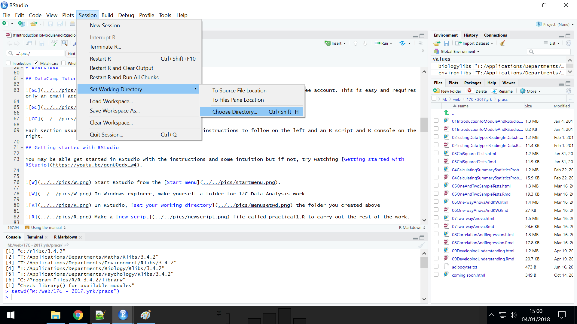
Start RStudio from the Start menu.

In RStudio, set your working directory to the folder you created previously for your 17C Data Analysis work.

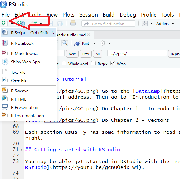
Make a new script file called workshop5.R to carry out the rest of the work.

You probably want to load the tidyverse with library(tidyverse).

Egg laying in parasitic wasps

The data in wasp.txt concern the egg-laying behaviour of a species of parasitic wasp, laying its eggs on a beetle larva. Wasps and other Hymenopterans (Ants and Bees) are haplo-diplod: unfertilised eggs are haploid and develop into males, whereas fertilised eggs are diploid and develop into females. Researchers wanted to know if mating status affected the time (in hours) the wasp takes to lay its eggs. Each row represents an individual wasp. The first column gives the time taken and the second column indicates whether they are mated or unmated.

Save a copy of the data file wasp.txt

Read in the data and check the structure

Do a quick plot of the data:

ggplot(data = wasp, aes(x = status, y = time)) +
  geom_violin()

Summarising the data

Find the means for each group. You may need to look this up Week 3: Testing, Data types and Reading in data

Create a data frame called waspsummary that contains the means, standard deviations, sample sizes and standard errors for the mated and unmated females. You may want to look this up in the lecture notes.

Selecting

Do you think this is a one/paired test or two-sample test?

Applying, interpreting and reporting

Carry out a two-sample t-test:

t.test(data = wasp,
       time ~ status,
       var.equal = T)

## 
##  Two Sample t-test
## 
## data:  time by status
## t = -3.1407, df = 58, p-value = 0.002653
## alternative hypothesis: true difference in means is not equal to 0
## 95 percent confidence interval:
##  -12.716797  -2.816536
## sample estimates:
##   mean in group mated mean in group unmated 
##              23.36667              31.13333

What do you conclude from the test? Write your conclusion in a form suitable for a report.

Check assumptions

We need to calculate the residuals – the difference between predicted (i.e., the group mean) and observed values. We can do this in two steps:

First by adding a column that holds the mean for the group each value belongs to by ‘merging’ the summary data into the raw data:

# add the group means to the data
wasp <- merge(wasp, waspsummary, by = "status")

I suggest you look at the wasp dataframe to see what this code has done.

Second by adding a column for each ‘residual’

# add the group means to the data
# add the residuals
wasp <- wasp %>%
  mutate(residual = time - mean)

Now we are ready to examine the distribution of the residuals.

Run a normality test:

shapiro.test(wasp$residual)

## 
##  Shapiro-Wilk normality test
## 
## data:  wasp$residual
## W = 0.9749, p-value = 0.2516

Usually, when we are doing statistical tests we ‘hope’ we will find significance. In this case, we hope it will not be significant. A non-significant result means that there is no significant difference between the distribution of the residuals and a normal distribution.

What do you conclude from the result of the normality tests?

Check the residuals are homogenously distributed (variance is the same in both groups):

ggplot(data = wasp,
       aes(x = mean, y = residual)) +
  geom_point()

There’s a bit of an outlier in one group but this looks ‘ok’.

Illustrating

We are going to create a figure like this:

In this figure, we have the data points themselves which are in wasp dataframe and the means and standard errors which are in the waspsummary dataframe. That is, we have two dataframes we want to plot. Here you will learn that dataframes and aesthetics can be specified within a geom_... (rather than in the ggplot()) if the geom only applies to some of the data you want to plot.

We will build the plot up in small steps but as you get more used to ggplot you’ll probably be able to create figures in fewer steps. Each time you run ggplot() you get a new plot, you are not actually adding to an existing plot.

First, create an empty plot:

ggplot()

Now add the data points:

ggplot() +
  geom_point(data = wasp, aes(x = status, y = time))

Notice how we have given the data argument and the aesthetics inside the geom. The variables status and time are in the wasp dataframe

So the data points don’t overlap, we can add some random jitter in the x direction:

ggplot() +
  geom_point(data = wasp, aes(x = status, y = time),
             position = position_jitter(width = 0.1, height = 0))

We’ve set the vertical jitter to 0 because, in contrast to the categorical x-axis, movement on the y-axis has meaning (time).

Let’s make the points a light grey:

ggplot() +
  geom_point(data = wasp, aes(x = status, y = time),
             position = position_jitter(width = 0.1, height = 0),
             colour = "grey50")

Now to add the errorbars. These go from one standard error below the mean to one standard error above the mean.

Add a geom_errorbar() for errorbars:

ggplot() +
  geom_point(data = wasp, aes(x = status, y = time),
             position = position_jitter(width = 0.1, height = 0),
             colour = "grey50") +
  geom_errorbar(data = waspsummary, 
                aes(x = status, ymin = mean - se, ymax = mean + se),
                width = 0.3)

We have specified the waspsummary dataframe and the variables status, mean and se are in that.

There are several ways you could add the mean. You could use geom_point() but I like to use errorbars that start and stop in the same place, the mean.

Add a geom_errorbar() for the mean:

ggplot() +
  geom_point(data = wasp, aes(x = status, y = time),
             position = position_jitter(width = 0.1, height = 0),
             colour = "grey50") +
  geom_errorbar(data = waspsummary, 
                aes(x = status, ymin = mean - se, ymax = mean + se),
                width = 0.3) +
  geom_errorbar(data = waspsummary, 
                aes(x = status, ymin = mean, ymax = mean),
                width = 0.3)

Alter the axis labels and limits:

ggplot() +
  geom_point(data = wasp, aes(x = status, y = time),
             position = position_jitter(width = 0.1, height = 0),
             colour = "grey50") +
  geom_errorbar(data = waspsummary, 
                aes(x = status, ymin = mean - se, ymax = mean + se),
                width = 0.3) +
  geom_errorbar(data = waspsummary, 
                aes(x = status, ymin = mean, ymax = mean),
                width = 0.3) +
  ylab("Time (hr)") +
  xlab(NULL) +
  ylim(0, 70)

And finally format the figure in a way that is more suitable for including in a report:

ggplot() +
  geom_point(data = wasp, aes(x = status, y = time),
             position = position_jitter(width = 0.1, height = 0),
             colour = "gray50") +
  geom_errorbar(data = waspsummary, 
                aes(x = status, ymin = mean - se, ymax = mean + se),
                width = 0.3) +
  geom_errorbar(data = waspsummary, 
                aes(x = status, ymin = mean, ymax = mean),
                width = 0.2) +
  ylab("Time (hr)") +
  xlab(NULL) +
  ylim(0, 70) +
  scale_x_discrete(labels = c("Mated", "Unmated")) +
  theme_classic()

Grouse Parasites

These data come from a sample of grouse shot in Scotland. The grouse livers were dissected and the number of individuals of a parasitic nematode were counted. We want to know if males and females have different infection rates.

males: 5, 16, 8, 64, 51, 11, 9, 7

females: 0, 2, 1, 3, 6, 10, 4, 12

Create dataframe for these data. Mine ended up like this . You might find it useful to look at workshop 2

Selecting

Do these data look normally distributed?

What is the null hypothesis?

What test do you suggest?

Applying, interpreting and reporting

Summarise the data by finding the median of each group.

## # A tibble: 2 x 2
##   sex     `median(nematodes)`
##   <chr>                 <dbl>
## 1 females                 3.5
## 2 males                  10

Carry out a two-sample Wilcoxon test (also known as a Mann-Whitney):

wilcox.test(data = grouse, nematodes ~ sex)

## 
##  Wilcoxon rank sum test
## 
## data:  nematodes by sex
## W = 10, p-value = 0.02067
## alternative hypothesis: true location shift is not equal to 0

What do you conclude from the test? Write your conclusion in a form suitable for a report.

Illustrating

A box plot is a usually good choice for illustrating a two-sample Wilcoxon test because it shows the median and interquartile range.

We can create a boxplot with:

ggplot(grouse, aes(x = sex, y = nematodes) ) +
  geom_boxplot() + 
  xlab("Sex") +
  ylab("Number of nematodes") +
  theme_classic()

Gene Expression

Researchers are interested in the expression levels of a particular set of 35 E.coli genes in response to heat stress. They measure the expression of the genes at 37 and 42 degrees C (labelled low and high temperature). These samples are not independent because we might expect there to be a relationship between expression at 37 and 42 degrees within a gene.

Selecting

What is the null hypothesis?

Save a copy of coliexp.txt

Read the data in

What is the appropriate parametric test?

Applying, interpreting and reporting

Now carry out a paired-sample t-test.

t.test(data = coliexp, expression ~ temperature, paired = T)

## 
##  Paired t-test
## 
## data:  expression by temperature
## t = 3.2039, df = 34, p-value = 0.002943
## alternative hypothesis: true difference in means is not equal to 0
## 95 percent confidence interval:
##  0.1123712 0.5021946
## sample estimates:
## mean of the differences 
##               0.3072829

State your conclusion from the test in a form suitable for including in a report. Make sure you give the direction of any signifcant effect.

Independent study

Analyses

Decide which test you should use to analyse the following data sets. In each case give the reasons for your choice of test and state the null hypothesis. Write your conclusions in a form suitable for including in a report. Can you make figures?

Plant Biotech

Some plant biotechnologists are trying to increase the quantity of omega 3 fatty acids in Cannabis sativa. They have developed a genetically modified line using genes from Linum usitatissimum (linseed). They grow 50 wild type and fifty modified plants to maturity, collect the seeds and determine the amount of omega 3 fatty acids. The data are in csativa.txt Do you think their modification has been successful?

Sheep diet

In order to investigate the effects of feeding fertilised grass to sheep, one of each pair of fourteen sets of twins was fed fertilised grass whilst the other was fed unfertilised grass and the adult weight of the sheep was recorded. The data are in sheep.txt . Is there difference in the effect of fertilised and unfertilised grass on sheep weight?

Reading

Wickham, H (2013). Tidy Data. Journal of Statistical Software.

The Code files

These contain answers and code even though they do not appear on the webpage itself.

Rmd file The Rmd file is the file I use to compile the practical. Rmd stands for R markdown allow R code and ordinary text to be inter weaved to produce well-formatted reports including webpages.

Plain script file This is plain script (.R) version of the practical

Script example

This is an example of a well formatted analysis script for the wasp data.

Script example

Objectives from previous sessions

Introduction to module and RStudio

to explain why we need statistical tests and the logic of hypothesis testing (MLO 1)
use the R command line as a calculator and to assign variables (MLO 3)
create and use the basic data types in R (MLO 3)
find their way around the RStudio windows (MLO 3)
create, use and save a script file to run r commands (MLO 3)
search and understand manual pages (MLO 3)

Testing, Data types and reading in data

to able to explain what response and explanatory variables are, distinguish between data types and describe how these impact choice of test (MLO 1 and 2)
demonstrate the process of hypothesis testing with an example and evaluate potential inferences (MLO 1 and 2)
read in data in to RStudio, create simple summaries and plots using manual pages where necessary (MLO 3)
create neat reports in Word which include text and figures (MLO 4)

Goodness of Fit and Contingency chi-squared tests

recognise when to use chi-squared Goodness of Fit and Contingency tests (MLO 2)
be able to carry out, interpret and report scientifically both types in R (MLO 3 and 4)

Calculating summary statistics, probabilities and confidence intervals

Explain the properties of ‘normal distributions’ and their use in statistics (MLO 1 and 2)
Define, select and calculate with R probabilities, quantiles and confidence intervals (MLO 3 and 4)

One- and two-sample t-tests and their non-parametric equivalents

Emma Rand

Introduction

Aims

Learning Outcomes

Philosophy

Slides

Exercises

Getting started

Egg laying in parasitic wasps

Summarising the data

Selecting

Applying, interpreting and reporting

Check assumptions

Illustrating

Grouse Parasites

Selecting

Applying, interpreting and reporting

Illustrating

Gene Expression

Selecting

Applying, interpreting and reporting

Independent study

Analyses

Plant Biotech

Sheep diet

Reading

The Code files

Script example

Objectives from previous sessions